MGMT 803, MBA@Rice, 2026

Neural networks

Kerry Back
J. Howard Creekmore Professor of Finance

This session

Inside a neural network
Training
Fine-tuning and LoRA

27 · Inside a neural network

One neuron

Part 1 described a neural network as a function with parameters.

A neuron weights the numbers coming into it, adds a bias, and passes the result through an activation function.

\[z = b + w_1 x_1 + w_2 x_2 \qquad\qquad h = f(z)\]

Weights

\(w_1\) and \(w_2\) set which inputs matter and how much. A negative weight subtracts.

Bias

\(b\) shifts the sum. With ReLU it sets how large the weighted inputs have to be before the neuron produces anything at all.

Two activation functions

Sigmoid

\[\sigma(z) = \frac{1}{1 + e^{-z}}\]

Output between 0 and 1. Used on an output neuron when the answer is a probability.

ReLU

\[\max(0,\, z)\]

Output 0, or the value itself. Used in hidden layers: cheaper, and the derivative does not shrink toward zero for large \(z\).

Why the activation is there

Without it

A weighted sum of weighted sums is another weighted sum. Stack a hundred linear layers and the whole network reduces to one linear function of the inputs.

With it

Each layer bends the function. Depth then adds capacity instead of repeating what a single layer could already do.

A small network

Two inputs, three neurons in a hidden layer, one output. Every input connects to every neuron in the next layer.

9 hidden layer: 3 biases and 3 × 2 weights

4 output: 1 bias and 3 weights

13 parameters to be chosen

The forward pass

The same pass in code

W1 = np.array([[0.5, 0.3], [-0.4, 0.6], [0.2, -0.3]])   # 3 neurons x 2 inputs
b1 = np.array([0.1, -0.2, 0.3])
W2 = np.array([0.7, -0.5, 0.8])
b2 = 0.2

x = np.array([1.2, -0.8])

h = sigmoid(W1 @ x + b1)      # hidden layer, 3 values
y = sigmoid(W2 @ h + b2)      # output, 1 value

W1 @ x is a matrix-vector product: one row per neuron, one multiply-add per weight. That product is the operation GPUs are built for.

The same arithmetic at scale

13 parameters in the network above

1 billion Gemma 3 1B, which runs on a laptop

100s of billions a frontier model

The arrangement differs: a transformer’s layers include attention, from Part 1, rather than a plain fully connected stack. Every unit in it still takes a weighted sum, adds a bias, and applies an activation.

28 · Training

What training chooses

Chosen by training

Every weight and every bias. The 13 numbers above, or the hundreds of billions in a frontier model.

Chosen by hand, before training

How many layers, how many neurons in each, which activation, how large a step to take.

The loss

Training needs one number to make smaller. For each example, compare what the network produced to the right answer.

Task	Output layer	Loss
Predict a quantity	one neuron, no activation	squared error
Predict a label	one neuron, sigmoid	cross-entropy
Predict one of many labels	one neuron per label, softmax	cross-entropy

A language model is the third row, with one label per token in the vocabulary. Next-token prediction is a classification problem with about 100,000 classes.

Gradient descent

Run a batch of examples forward and compute the loss.
Find the derivative of the loss with respect to every parameter.
Move each parameter a small step against its derivative.
Repeat.

The size of that step is the learning rate. The notebook later in this session uses 2e-4.

Backpropagation

Step 2 is the one that needs an algorithm.

One parameter at a time

Nudge a weight, run the whole network forward again, see how the loss moved. With a billion parameters that is a billion forward passes for one step.

Backpropagation

Apply the chain rule from the loss backward through the layers. One backward pass yields the derivative for every parameter, at roughly the cost of one forward pass.

Held-out data

Training set

The examples the parameters are fitted to. Loss here keeps falling for as long as you keep training.

Test set

Examples held back and never fitted. Loss here stops falling, then rises, while training loss is still improving.

With enough parameters a network can fit its training examples exactly and still do no better than chance on new ones.

29 · Fine-tuning and LoRA

Three ways to change what a model does

	What changes	Use when
Prompting	the text sent with the request	the model can do the job and needs telling
Retrieval	documents put into the context, from Part 6	it needs facts it was not trained on
Fine-tuning	the weights	the behavior has to change: a format, a style, a judgment call

Fine-tuning does not add knowledge reliably.

When fine-tuning is worth it

A fixed output format

A label, a JSON record, a field in another system. Prompting gets the format most of the time.

Many examples, one narrow job

Thousands of labeled cases already exist, and the job will run millions of times.

Cost per call

A small fine-tuned model can match a large prompted one on one narrow task, at a fraction of the cost per call.

Distillation

Run a frontier model on your inputs and keep its answers.
Treat those answers as labels.
Fine-tune a small open-weights model on them.

Part 6 covered where this runs into a provider’s terms. Read them before doing it with a commercial model’s output.

Full fine-tuning and LoRA

Full fine-tuning

Update every parameter. Needs GPU memory for the weights, their gradients and the optimizer state, and produces a complete copy of the model.

LoRA

Freeze the original weights. Train two small matrices per layer instead. In the notebook later in this session, that is under 0.1% of the model’s parameters.

Hu et al., 2021: low-rank adaptation.

The weight matrix

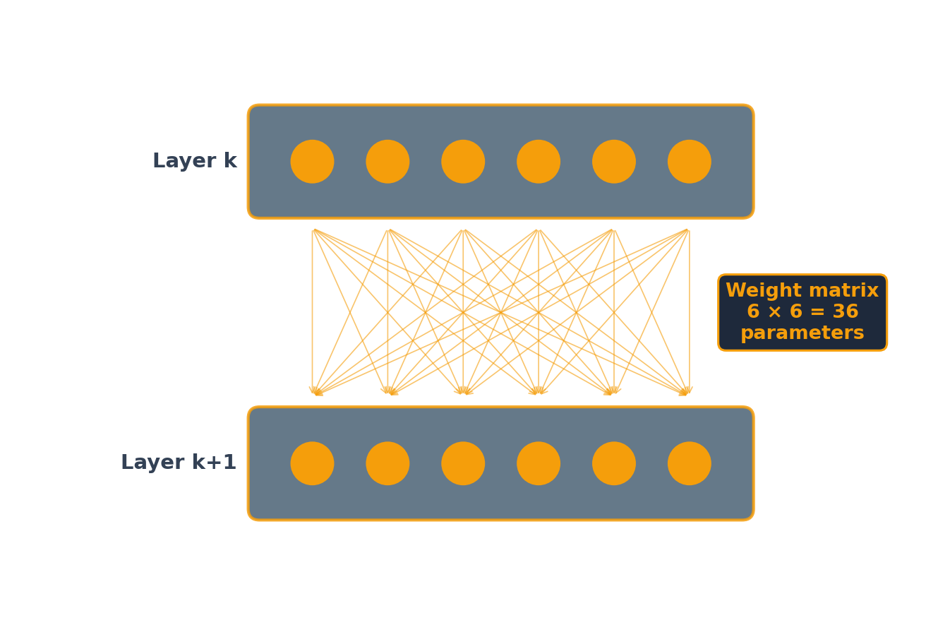
Six neurons feeding six neurons: 36 weights, one per connection. Full fine-tuning retrains all of them.

The low-rank path

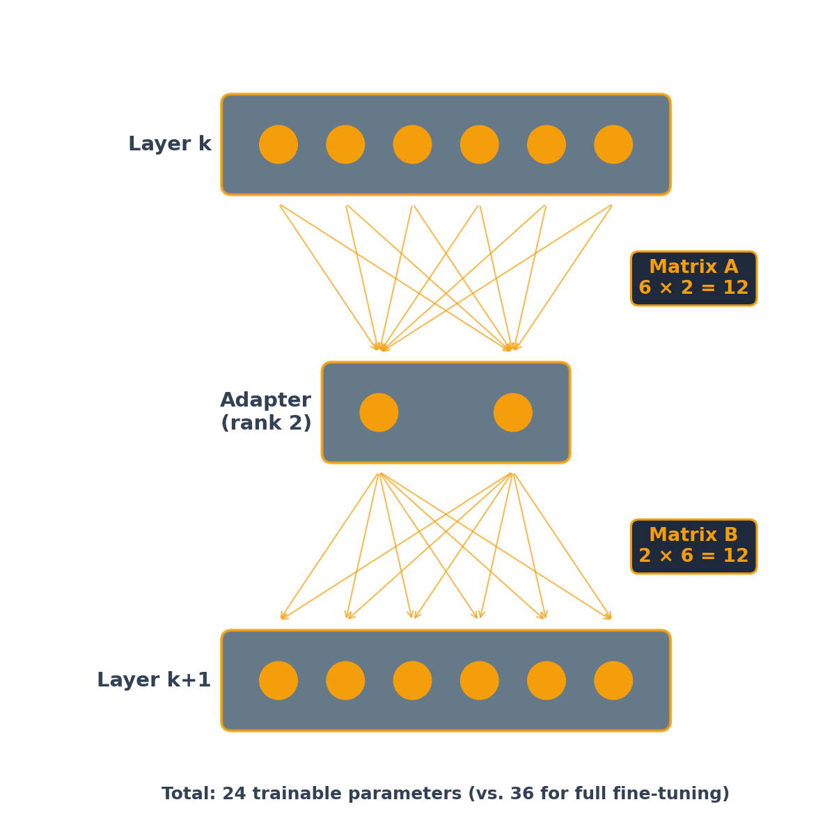
The 36 frozen connections are not drawn. The trained path runs through two neurons: rank 2.

LoRA: the arithmetic

\(A\) compresses the input down to the rank and \(B\) expands it back up, so the product \(BA\) has the same shape as the original weight matrix \(W\) and can be added to it:

\[W' = W + BA\]

There is no activation function in the adapter path, which is why \(BA\) is a matrix and the addition is possible. Once merged, the model has the architecture and the speed it had before.

At real scale

The six-by-six picture is a diagram. A transformer’s layers are 4096 × 4096 and larger.

16.8M parameters in one 4096 × 4096 layer

131K trained by a rank-16 adapter on it

128× fewer parameters to train

The adapter is also what you store and ship: a file of megabytes, where full fine-tuning leaves you a second copy of the whole model.

QLoRA

The base model, quantized

Weights stored at 4 bits instead of 16. Gemma 3 1B goes from about 2 GB to about 800 MB.

Adapters on top of it

The frozen weights are read at 4 bits; the small matrices train at full precision. A 70-billion-parameter model fits on one 48 GB GPU.

Dettmers et al., 2023. This is what puts fine-tuning on a free Colab T4, which has 16 GB.

Hands-on: fine-tune Gemma 3 1B

Google Colab · free T4 GPU · about 15 minutes of training

Load Gemma 3 1B at 4 bits.
Attach rank-16 adapters to the attention layers, q_proj and v_proj only.
Train on Financial PhraseBank: 2,264 news sentences that every annotator labeled the same way, positive, negative or neutral.
Run three test sentences through the model before and after.

Open the notebook in Colab

Needs a Hugging Face account, a read token, and Google’s Gemma license accepted at huggingface.co/google/gemma-3-1b-it.

Breakout exercise

Run the notebook as far as the baseline cell, and read what the base model says about the three test sentences.
Train, then compare the answers before and after.
The base model is about 2 GB and the saved adapter is 14 MB. Say what has to be on the serving machine for the fine-tuned model to answer, and what changes if you merge the adapter into the weights instead.